
Linux for Data Scientists, Part 1

Everyone’s path to data science is different. Some of my colleagues have backgrounds in fields like anthropology, psychology, philosophy, physics, and finance. But to be reductionist, most people enter the data science world from one of two directions: mathematics/statistics and computer science.
I majored in computer science in my undergraduate career, and my strengths lie there. Because of my background, some of my mathematically-inclined colleagues have solicited my advice on how to become more adept with computers. Personally, I believe that acquiring a base level of computer knowledge can make a data scientist several times more productive (especially on routine projects). This efficiency is gained primarily in two ways: coming to understand the Linux environment in which you work, and becoming skilled at manipulating that environment. This distinction may seem arbitrary, but it’s important to draw the line between knowing and using; the latter without the former can lead to major mistakes.
You may notice I’ve assumed above that your environment is running Linux. While I am myself a fan of the Linux family of operating systems, this isn’t just a personal bias. The vast majority of serious computing platforms run on Linux, as do nearly all web servers. Linux has become the de facto standard for production-quality and high-performance software, especially in data science. For this reason, this post will assume that your regular environment is running Linux, though MacOS supports many of these features as well.
Getting down to business, this walkthrough assumes you already know the very basics of Linux, such as:
How to connect to a Linux server
How to move files to a Linux server from your local computer, and vice versa
Knowing your environment
Looking under the hood is daunting, but you can’t unlock the full power of your tools (or your own skills) until you know your environment.
This is especially true when your code fails or runs slowly. Where is the bottleneck? It takes a bit of computer know-how to figure this out, but once you do, significant performance improvements become attainable. For example, if you determine that your program is CPU-bound, you can take steps to parallelize your algorithm. If memory is the problem, you may decide that you need to implement your algorithm in a distributed environment like Spark.
top
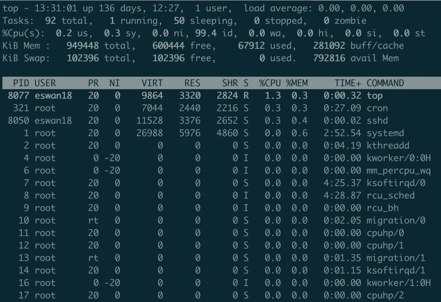
First, let me introduce top, a great one-stop shop for information about what’s happening on your machine.
top shows you the processes running on your machine, ordered by resource consumption (thus the name). For most users, the important columns are %CPU and %MEM – these indicate the percent of CPU time being used and the percent of memory being occupied by the program, respectively. By default, programs are ordered by %CPU.
Many users run top every day in its basic form, but aren’t familiar with some simple ways to get more detailed information. Pressing M (capital M, to be clear) will reorder the list by %MEM. Pressing 1 will break down resource consumption at the core level instead of the program level. This can be useful to determine whether further parallelization could make your scripts faster. u followed by a username and will limit the list to only processes run by that user. Last, q returns you to the command prompt.
As a general rule of thumb, top should be the first tool you turn to when diagnosing one of your own programs.
free
When you want a very high-level view of the memory situation on a Linux machine, use free. When deployed with the -h flag (for human-readable, meaning that raw counts of bytes should be converted to megabytes, gigabytes, etc.), free will display a simple readout of how much memory is used and available on your system.
What you should look at is total (how much memory your machine has in total), used (how much memory is in use), and available (how much memory is left for you to use). You may notice that the free column displays a different count than the available column – this is not unusual. Some memory is not fully freed by the operating system until necessary, but it is available if needed.
Note that free, unlike all of the other commands in this article, is not implemented in MacOS. See this old StackExchange question if you’re interested.
du
Short for disk usage, du is extremely useful for estimating the size of directories. You may have noticed that running ls -l on a directory shows the directory as only consuming a tiny amount of disk space – often 4K or less.
Of course, the items in this directory might be using more than 4096 bytes; but you asked Linux for the size of the directory itself, and it reported to you how much space the abstraction of a “directory” actually requires. Since Linux treats everything as a file, a directory is just a small file that points to other files (whatever that directory contains).
However, you’re a human and the size of a file that points to other files is probably not what you were after. It’s here that du is a real asset. du will do the hard work of totalling all the contents of a directory, recursively, so you can accurately assess how much space a directory is taking on disk. As with free, du is best used with the -h flag so that its readout is in megabytes or gigabytes as appropriate. And to tell du that we want just a single output per input (not the size of every single thing inside a directory, listed), we also want to pass the -s flag for summarize. Thus, the full command we will run is du -sh <directory_name>.
408 kilobytes. A lot more than 4.
df
df stands for disk free. Because of their similar names, df and du are easily confused. However, df is for monitoring disk space at the filesystem level. Most enterprise servers are actually comprised of several separate but linked filesystems. Without getting into the nitty gritty details of filesystems, it’s just important to know that each entry displayed by df is a separate area with a finite storage limit – and it’s possible that one area can fill up entirely, preventing you from creating new files or modifying current ones there.
Run df with our friend -h to get a nice summary of the filesystems on a server.
The Mounted on column shows where the relevant filesystem is “mounted” on our current system. While something like /dev may look like any other folder, in this case it is actually a separate filesystem. That means that we could run out of space in /dev but still have room on the rest of the server – or vice versa.
It’s common for enterprises to link several servers by mounting a single filesystem on all of them, and then making the actual per-server disk space very small. But because many configuration files live in the /home directory, the individual servers may still run out of space and produce strange errors when unable to update configurations. This is when you should take a look at df to assess what’s going on.
Working with Files and Text
While it’s tempting to stay within the seemingly-friendly realm of GUI-based applications, becoming skilled at operating directly in the terminal can make you massively faster at typical tasks. The best example of this truth can be seen in Vim, a famously powerful but esoteric text editor. I highly recommend becoming a Vim power user, but I won’t talk about it here; the subject merits an entire article to itself. Other (simpler) command line tools have less-daunting learning curves than Vim, but still offer significant gains in productivity.
wc
The simplest command in our toolbox is wc. Its name stands for word count, but actually wc counts characters and lines as well as words. Invoke it with wc .
This file contains 95 lines, 308 words, and 3467 characters. Because this output is a little bit noisy, and usually a line count is enough, wc is commonly used with the -l flag to just return a line count.
grep
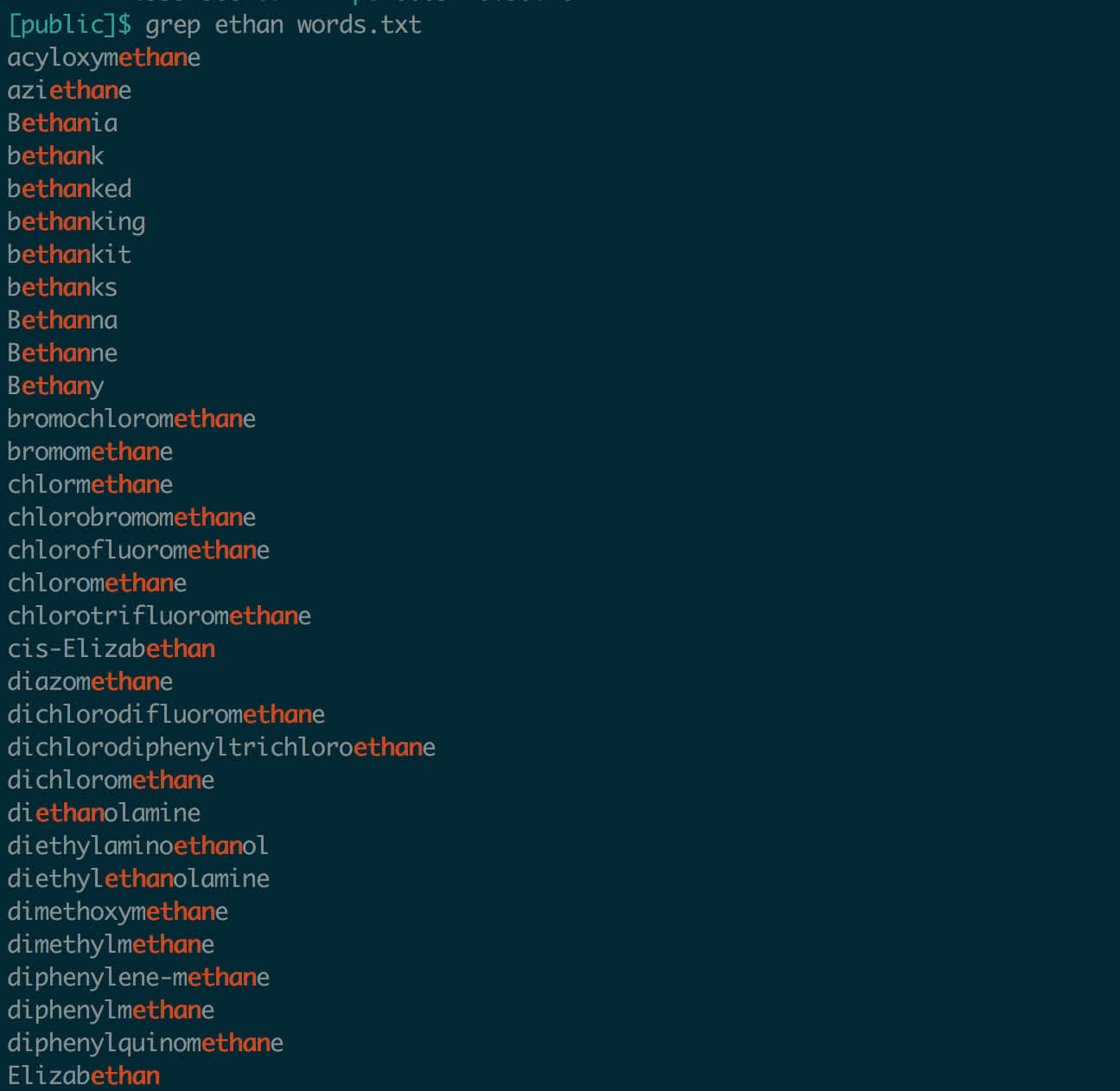
grep might be the most famous command line tool. It’s a superpowered text-searching utility. The name comes from Globally search a Regular Expression and Print. In its simplest form, grep , it will look through a file and find all instances of a certain string. Let’s search a dictionary of valid words for my name.
Who knew I was in the dictionary?
Adding the -i flag makes your search case-insensitive (like most things Linux, grep is case-sensitive by default). When dealing with prose, like readme files, this is very handy. There are many, many more flags available, and grep can handle more complicated match strings, called regular expressions. Consult the man page (man grep) for the details.
awk
awk bears the distinction of being one of the least-intuitively named command line tools. The name is just an abbreviation for its authors: Aho, Weinberger, and Kernighan.
awk is essentially a very simple programming language optimized for dealing with delimited files (e.g. CSVs, TSVs). It’s Turing Complete, and in theory you could do pretty much anything with it, including data science. But please don’t.
The time for awk is when you have a text file that you want to manipulate like a table. If you find yourself thinking* I need to see the third field of each line*, or What’s the sum of the first four fields of this file?, you’re entering awk territory.
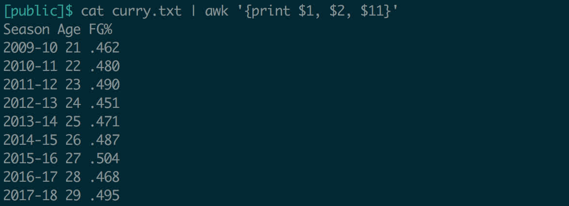
Invoke it with__ awk __. awk can be a little intimidating at first, so let’s look at an example. Here’s a file of Steph Curry’s stats by season, from Basketball Reference. Columns are separated by spaces.
Fields in awk are referenced by a dollar sign and their position; $1 is the first field, $4 is the fourth field, etc. (Note that awk is not zero-indexed!) Always issue your command in quotes to tell the shell not to parse it and instead to pass the whole string to awk. Since right now we want our command to run line-by-line, we will use curly braces within the quotes. If you wanted to see just the first column of each row, the command would be '{print $1}'. The first and the fifth field would be '{print $1, $5}'.
Okay, so we can extract columns. This comes in handy when examining big files. But we can do more! What if we wanted to know how many free throws plus field goal attempts Curry has recorded each season?
Why is the first line zero? Because the first line of the file was headers, we tried to add “FGA” to “FTA”.awk knows that these aren’t numbers, and so it just treats them as zeros.
This file was space-delimited, which obviously plays well with awk. How would we handle a file delimited by a different character? Fortunately, this is simple: the -F flag, for field separator, takes an argument that awk will use to split the file. To be safe, pass the argument in quotes.
Let’s split the Curry data on a dash instead of spaces, and print the first field.
awk returned each line up to the first dash, as expected. Using this technique, you can use awk on a huge variety of flat files.
We’ve barely scratched the surface of what awk can do, but this is a good starting point.
sed
sed stands for Stream EDitor. Like awk, it’s Turing Complete and extremely powerful. For now, we’re just going to focus on its find-and-replace abilities.
The basic syntax for this is sed 's/<find_pattern>/<replace_pattern>/g' . The ‘s’ stands for substitute, a more formal term for find-and-replace. The ‘g’ is for global – without it, sed will just replace the first occurence of your find pattern on each line.
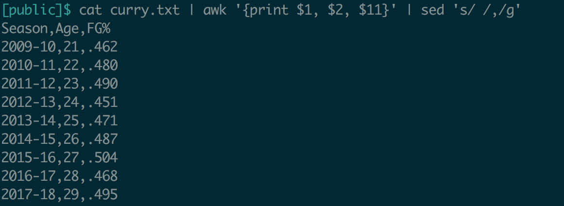
Let’s try to modify the Curry data, to make it comma-delimited instead of space-delimited.
This output is very useful as long as we’re willing to copy and paste it. What if we wanted to actually modify the input file itself? sed supports this feature, using the -i (for in-place) flag. So sed -i 's/ /,/g' curry.txt would update the file to be a CSV – although if we wanted the file extension to reflect this change, we’d have to handle that ourselves.
Again, as with awk, sed has many many useful options and modes. At the beginning, though, try to just get comfortable with this functionality and research more options as you need them.
| (pipe)
We’ve gone through a lot of information so far, and maybe it doesn’t even seem that useful. How often do I only need to view a column or search for a word?, you might think, I need to do all of these things at the same time, sometimes repeatedly, which I can only do in a more fully-featured tool like Python or SQL.
But no! In fact, the simplicity of these tools is perhaps their greatest asset. Unix, the family of operatings systems from which Linux descends, is built on modularity. Each tool is to do one thing, and only one thing, and do it well. Tools can be chained together using an operator called the pipe, which takes output from one command and sends it to another as input.
Before demonstrating the pipe, I need to introduce another tool: cat. Short for concatenate, cat simply takes a filename and outputs its contents. Sticking with the Curry data:
cat, on the surface, seems like a superfluous tool. However, with the pipe at your disposal, it becomes highly useful:
Take a look at what’s going on here. Unlike when we used awk above, we didn’t need to provide it with a filename. Instead, it took the output of the command before it (cat curry.txt) and used that as its input. What if we wanted to make this output comma-delimited?
Pipes allow you to chain together as many commands as you’d like, using each command to transform the output of the last. This unlocks an enormous amount of power without requiring you to import data into a specialized tool. Remember, data movement is often the slowest part of a process, so operating directly on the filesystem can be extremely efficient.
Piping isn’t limited strictly to operations on files. Remember df? What if we just wanted to see how much space is available on the home mount?
We just used grep to search for lines that contain ‘home’ in the output of df -h. Linux is designed with these types of operations in mind, so this logical chaining works surprisingly smoothly. Wondering how many years Curry played for Golden State?
This is a very common technique. Use a tool like grep to find rows of your data that meet a condition, and then use__ wc -l__ to count how many rows were selected.
With practice, you’ll start thinking in terms of piping. Complex operations become easier to break down into their components and corresponding tools required.
> (chevron)
The last feature I’ll talk about is the chevron (sometimes called “waka” in computer-speak). Both chevron directions (< and >) are supported, but the right-pointing one is generally more useful. > is used for output redirection: sending what usually displays on screen into a file instead.
Let’s start with an example:
This operation produces no output. What happened?
Aha! So we just created a file with the output of__ free -h__. This could be useful for regularly logging how much memory is in use on the server.
Output redirection is especially useful when doing file manipulation. Above, in the pipe section, we extracted Curry’s field goal percentage each year and made it comma-delimited. You might want to save this modified data in a new file.
Suddenly, we’ve created a CSV of this data on disk, in one line. This is the power of the pipe and output redirection used in tandem.
Wrapping Up
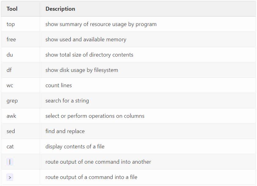
Because this is a lot to digest, I want to close with a cheat sheet. Below is a table explaining, very briefly, what each tool we’ve discussed is used for.
With these tools in your belt, many operations typically reserved for high-level technologies are possible in Linux. You can save time that you once spent copying files locally, modifying them, and then copying them back to the server.
Whenever you are in need (or are simply interested) in more information about how a command works, look to to the man pages (short for manual). Though you might expect man pages to be terse and dry, in general they’re very readable and extremely comprehensive. A good place to begin would be man wc, which calls up a fairly short and digestible entry.
In the near future, I hope to publish Part 2, covering some more advanced patterns of working in Linux: using head and tail, simple regular expressions, and basic bash syntax.
Visit our knowledge hub
See what you can learn from our latest posts.







![[DO NOT DELETE] 8451-PR header 4000x2000 shutterstock 2146084959 po](https://images.ctfassets.net/c23k8ps4z1xm/CUmZcselsJUhnLz6rQuj2/0e48394e72423bb1073bf8bb6cf75974/8451-PR_header_4000x2000_shutterstock_2146084959_po.jpg?w=328&h=232&fit=fill)